In the present work, we selected 85 key proteins in Alzheimer's disease. For further details about the target see the primary citation here. For each AD key protein, using the XGBoost classification and regression algorithm[1], three different ML models were built and then evaluated based on balanced accuracy, precision and F1 score metrics, respectively. Balanced Accuracy is the arithmetic means of sensitivity and specificity and is used in both binary and multi-class classification ML models. It is recommended to be used when dealing with imbalanced data. Precision quantifies the number of correct positive predictions by calculating the accuracy of the true positive. F1 score was selected because it integrates precision and recall into a single metric to gain a better understanding of model performance. F1 score is commonly used as an evaluation metric in binary ML modes. These metrics are widely recommended in the literature for studies that require accurate interpretation of model effectiveness across classes[2].

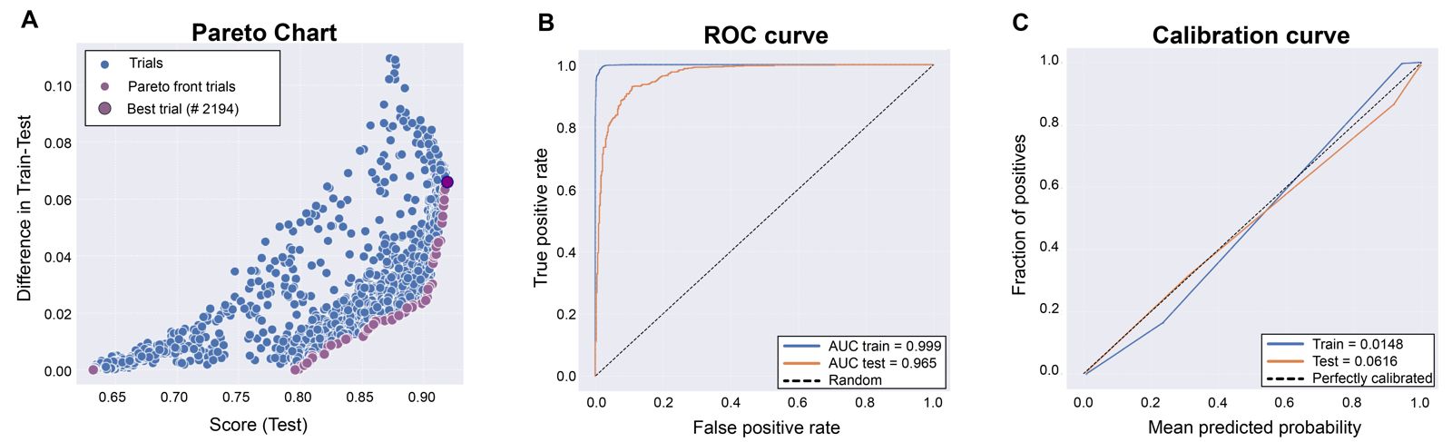
As an example, the validation of the ML model built for BACE1 (beta secretase-1) protein (Uniprot ID: P56817) evaluated with the precision metric is shown in Figure 1. 2902 active and 1690 inactive compounds were used to build ~3000 models for each run. We use 75% of the molecules for model construction and fitting, while the remaining 25% constituted the test set. The data partitioning was conducted using a random selection method with a fixed seed, thereby ensuring the reproducibility of these results in subsequent studies. This approach guarantees that the same data split will be replicated consistently, facilitating the validation and comparison of models in future research endeavors. The models were optimized using Optuna and to select the best model we used the Pareto optimization approach[3], that allow us to minimize the discrepancy between training and validation results, and maximize performance based on the precision evaluation metric. Figure 1A shows the Pareto chart with the best model selected after optimization. The XGBoost parameters of the best model in this case are: alpha = 1.0545, colsample_bytree = 0.5502, gamma = 0.1833, lambda = 1.8003, learning_rate = 0.0579, max_depth = 10.0, min_child_weigth = 1.0, n_estimators = 632.0, reg_alpha = 0.5484, reg_lambda = 0.3758, scale_pos_weigth = 1.118, and subsample = 0.8801. To illustrate the diagnostic ability of the ML BACE1 model evaluated with the precision metric, we plotted sensitivity against the specificity using receiver operating characteristic (ROC) curve, and then calculated the area under the curve (AUC - values between 0 and 1, the higher the better) for both the train and test sets (Figure 1B). AUC describes the probability of the ML model to rank a randomly chosen positive instance higher than a negative one. In addition, to know whether the model is reliable or not, the calibration curve (or reliability diagram) was plotted (Figure 1C). This curve compares how well the probabilistic predictions of our binary ML model are calibrated for both test and trains sets. Calibration curves that are closer to the diagonal indicate that the ML model is well calibrated.

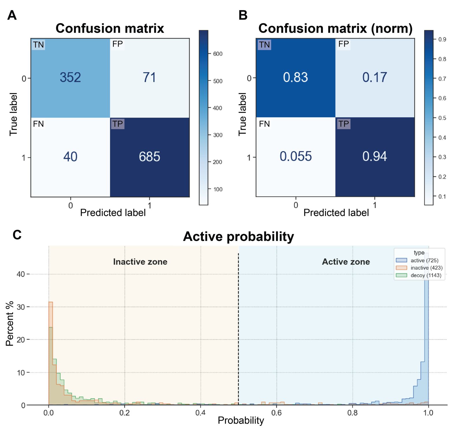
Afterwards, to test the BACE1-ML model we use the 25% of the remaining BACE1 active/inactive molecules and calculated the confusion matrix. This predictive analysis tool provides a structure comparison between true values with model predictive values, and it can be employed to evaluate different metrics used in the models. Within the matrix, four key variables characterize the classification process: True Positive (TP), True Negative (TN), False Positive (FP), and False Negative (FN) (Figure 2A). TP is when the positive data is classified as positive. TN is when the negative data is classified as negative. FP is when the negative data is classified as positive, and FN is when the positive data is classified as negative. Figure 2B illustrates a normalized confusion matrix derived from the BACE1-ML model. The data indicates that 83% of inactive compounds are correctly identified as such, while 94% of active compounds are correctly classified as active. Conversely, only 17% of inactive compounds are incorrectly classified as actives, and a minimal 0.55% of active compounds are erroneously classified as inactive. This matrix provides a quantitative overview of the model's classification performance, highlighting its ability to correctly identify both positive and negative instances, as well as its misclassification rates.

To gain further insight into this information, Figure 2C illustrates a bar plot divided into two distinct zones: inactive and active. This representation demonstrates that decoys and inactive compounds are predominantly located in the inactive zone (as expected), which aligns with the findings of the confusion matrix. Likewise, most active compounds are situated within the active zone. While there are instances where decoys and inactive compounds are classified as active, such occurrences are minimal. This visual representation provides a clear illustration of how the model's classification aligns with the distribution of compounds into active and inactive categories, corroborating the insights derived from the confusion matrix analysis.

To access all the data derived from the construction and validation see the details in the list on the right panel.

References

1. Tarwidi, D.; Pudjaprasetya, S. R.; Adytia, D.; Apri, M. An Optimized XGBoost-Based Machine Learning Method for Predicting Wave Run-up on a Sloping Beach. MethodsX 2023, 10, 102119.
2. He, H.; Garcia, E. A. Learning from Imbalanced Data. IEEE Trans. Knowl. Data Eng. 2009, 21 (9), 1263–1284.
3. Chen, Y.-S.; Chong, P. P.; Tong, M. Y. Mathematical and Computer Modelling of the Pareto Principle. Math. Comput. Model. 1994, 19 (9), 61–80.